Chapter 5 Option 3: Operating the model from your own machine
The Shiny (Chang et al. 2021) web application and stand-alone R code for implementation of the HWP model are available on GitHub for download. To run the files you will need to have R and RStudio installed on your computer. Both are free. R is the base program that executes the code; RStudio is an IDE, or Integrated Development Environment, that brings ease and power to using R. You will operate R through RStudio.
This chapter explains how to download or clone the GitHub repository and then describes all of the files in the repository. It then provides direction for running the Shiny app directly from your machine, followed by instructions for running the stand-alone R code from your computer. Finally, it describes how to use some downloaded code for appending extra harvest data to your input file.
5.1 R, RStudio, GitHub, and downloading the files
There are two ways to download all of the code and associated files. You can either download a zip file (~ 20MB) or clone the GitHub repository. If you clone the repository you can easily update the code from the GitHub site in the future.
5.1.1 Compressed file download
To obtain the compressed file, go to the GitHub repository, click the green “Code” button above the list of files, and then select the “Download Zip” option (see Figure 5.1). Unzip the folder on your machine and then check out the file structure and follow these directions for running the Shiny code and these for running the stand-alone version.
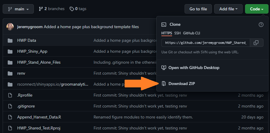
Figure 5.1: GitHub repository location for downloading the compressed files.
5.1.2 Clone the GitHub repository
To successfully clone the repository, you will need to have a program called Git installed on your computer. It may already be installed. There is a bit of a learning curve to getting Git up and going, as well as connecting to GitHub through RStudio. However, there are helpful websites that can smooth the way:
If you are not already using GitHub or similar, getting Git/GitHub/RProject set up may take an hour or two. I recommend reading through Happy Git website carefully and following its instructions. Going slowly is going quickly. You will also need to create a GitHub account.
Once you have Git set up on your machine and have verified that it is doing what you want you are ready to clone the repository. The following is based on Chapter 16 in Happy Git and Github (specifically 16.2), and assumes that your RStudio can connect to GitHub:
1. Select a location on your computer where you would like a folder containing the code to be placed.
2. Start R studio.
3. Select the following menu options: File > New Project > Version Control > Git
4. In the “repository URL” paste the URL of the HWP model’s GitHub repository: https://github.com/jeremygroom/HWP-C-vR.git
This will automatically populate the blank below the URL with the project name (HWP-C-vR).
5. Click “Create Project”
RStudio will now open the HWP-C-vR.Rproj file for you. You are ready to run the code. But first, we describe the files you’ve downloaded.
5.2 File structure
/HWP-C-vR/
This folder contains all files associated with the model, including template data, the Shiny application, the stand-alone code and folders, R environment controls, and the RStudio project that runs it all.
HWP-C-vR.Rproj: Open this to operate the Shiny app or stand-alone from your computer.
app.r: This is the main code file that runs the Shiny application.
HWP_Stand_Alone_Code.R: This is the main code file for running the stand-alone HWP model.
Append_Harvest_Data.R: This code will append new harvest data to your existing data file.
README.md: This file may contain some information about the GitHub version.
renv.loc: R environment information.
/HWP-C-vR/HWP Data/
This folder contains Oregon, California, and Washington data that may be uploaded into the app, test data for exploring the model’s functionality, and templates for constructing input files for elsewhere in the United States.
/HWP-C-vR/HWP Data/ExistingData/
This folder contains data files that may be loaded into the app or into the stand-alone model. The files include a harvest time series and timber and primary product ratios developed for these state-level inventories
CA_Inputs_HWP_Model.xlsx, Oregon_Inputs_HWP_Model.xlsx: These file contains the California and Oregon data already loaded in the app.
WA_Inputs_HWP_Model.xlsx: This file contains data for Washington State.
/HWP-C-vR/HWP Data/ModelExploration/
This folder contains files that allow the user to experience the app under different data scenarios (e.g., no ownership data) and practice appending additional data to existing files.
bogus.xlsx: This file will cause the QA check to halt the processing of the data and produce a warning.
CA_DiscardEnergyCapture_Test: This file contains the California data. The worksheet for discard fates (Section 4.2.2.10) is altered from 1980 and beyond to include a fraction of Discard Energy Capture (DEC).
OR_no_owner.xlsx: This file contains only total data for Oregon and lacks any ownership information.
Oregon_MBF_2019.xlsx: This file is not an input file. It contains two rows of additional Oregon harvest data for 2018 and 2019. Users may practice appending this harvest data to the current Oregon harvest data (1906 - 2017) with provided code (Section 5.5).
Oregon_MBF_2019v2.xlsx: Same as above, but this version includes all available Oregon harvest data (1906 - 2019).
/HWP-C-vR/HWP Data/Templates/
This folder contains sub-folders that direct users to Excel templates that they can use when building their input file.
/HWP-C-vR/HWP Data/HWP Data.zip/
This file contains compressed versions of the ExistingData and Templates folders for user download from the app.
HWP_Shiny_App/www/
This file only contains the Groom Analytics LLC logo for the application.
HWP_Shiny_App/R_code_data/
Most of the code that the Shiny application and stand-alone HWP model depend upon is in this folder:
dl_module.R: Shiny module that allows figures to be downloaded.
global.r: Initial code for reading in data for the Shiny application.
HWP.CA.output.rds, HWP.OR.output.rds: prepared data files that the Shiny application automatically imports to populate its figures.
HWP_Model_Function.r: This is the raw code for the HWP model, as is run by the stand-alone and the Shiny application. Note that simplified versions of this code are used for the Sankey diagram (located in PlotFunctions1.r) and the Monte Carlo simulation (see MC_Code.R).
HWP_Model_Prep.R: Code that extracts values from imported data and prepares them for entry into the HWP model functions.
HWP_Output_Prep.R: Code that simplifies variable names from HWP model function output.
HWP_Tables_Code.R: Generates output tables (CSV files) that the user can use to recreate plots. The Shiny application has a button that will appear on the Upload Data selection that allows users to download the tables. The stand-alone code also uses this code to populate its own folder for tables (see below).
LakePic_MC2.png, ShrubPic3.png: Pretty pictures for populating figure space when user data are not available.
MC_Code.R: This code runs the Monte Carlo simulation using user data. It is used by the Shiny application and the stand-alone model.
ModelRunPage.R: This module produces the Upload Data page for the Shiny application.
Plot modules. Each of these provides the code to run individual Shiny figure tabs:
- Plot_AnNetChCStor_Module.R: Produces the Annual Net Change in Carbon Storage tab underneath the header Carbon Storage and Emissions.
- Plot_AnnTimHarvest_Module.R: Produces the Annual Timber Harvest tab underneath the header Timber Harvest Summaries.
- Plot_CStorEm_Module.R: Produces the Carbon Storage and Emissions tab underneath the header Carbon Storage and Emissions.
- Plot_CStorOwn_Module.R: Produces the Carbon Storage by Ownership tab underneath the header Carbon Storage and Emissions.
- Plot_FateHarvC_Module.R: Produces the Fate of Harvested Carbon tab underneath the header Timber Harvest Summaries.
- Plot_MCest_Module.R: Produces the Monte Carlo Estimates tab underneath the header Carbon Storage and Emissions.
- Plot_HarvFuncLS_Module.R: Produces the Harvest by Functional Lifespan tab underneath the header Timber Harvest Summaries.
- Plot_AnNetChCStor_Module.R: Produces the Annual Net Change in Carbon Storage tab underneath the header Carbon Storage and Emissions.
PlotFunctions1.r: This code contains many of the functions used repeatedly by figures and the HWP model variants (standard HWP, Monte Carlo, and Sankey). It also contains the Sankey HWP model function. This code is source by the Shiny application and the stand-alone model.
QA_Code_Shiny.r: This code runs a Quality Assurance procedure on imported data. It verifies that the data are formatted correctly for entry into the HWP and Monte Carlo models. For more detail on the quality assurance procedure, see Section 4.3.
/HWP_Stand_Alone_Files/Arrays/
This folder serves as a destination for the arrays generated by the stand-alone code, given that the user’s data file indicates that arrays should be generated. The .gitignore file prevents the source code from uploading the arrays to GitHub.
/HWP_Stand_Alone_Files/QAQC_Reports/
This folder contains the error report (Error_Report.csv) generated by the stand-alone code’s call to QA_Code_Shiny.r. The .gitignore file prevents the source code from uploading any error reports in this folder to GitHub.
/HWP_Stand_Alone_Files/Standalone_R_files/
This folder contains two code files, MC_Tables.R and Sankey_Code.r. If the user indicates that the stand-alone code should generate tables of the Monte Carlo outcome, the MC_Tables.R file generates the tables. If the user indicates that the stand-alone code should generate a Sankey figure the Sankey_Code.r file will do so.
/HWP_Stand_Alone_Files/Tables/
This folder serves as a destination for tables generated by the stand-alone code, given that the user’s data file indicates that arrays should be generated. The tables are the same as those generated by the Shiny application after the user has run the HWP model on their own data and then selected the button that generates the tables. The .gitignore file prevents the source code from uploading any tables in the folder to GitHub.
/renv/
This folder contains R environment variables that the Shiny application (app.r) and stand-alone model (HWP_Stand_Alone_Code.R) rely upon. The environmental variables include version information for R and the libraries used. The user can ignore this folder.
/rsconnect/
This folder contains shinyapps.io deployment information. The user can ignore this folder.
5.3 Running the Shiny app from your computer
Open the code in RStudio. Launch the RStudio project by opening the project file HWP-C-vR.Rproj from within its folder. Within RStudio select from the menu File > Open File… . Select the file app.r and click on the Open button.
Run the code in RStudio. Here we run all of the code in the app.r file. There are several ways to do this. One way is to click on the code itself inside the code window, select all of the code (ctrl+A on a PC, apple+A on a Mac), and then ctrl+Enter (or apple+Enter) to run everything. Or, go to the menu item and select Code > Source.
Once you have run the Shiny application code, RStudio will display the application in its own window. A button at the top of the window will allow you to open the application in your own browser, but this isn’t necessary. The application should function as it does online when run from the Shinyapps.io server.
5.3.1 Details on running and editing the code
Users can run one or more lines of code by highlighting them and pressing ctrl-Enter or apple-Enter, or from the RStudio menu selecting Code > Run Selected Line(s).
The first line of the app.r or HWP_Stand_Alone_Code.R is: renv::restore(). The first time you run this line on its own or when running all of the code, the project file will (with your permission) download all versions of all libraries and the R instance used to run the app (Ushey 2022). It takes a little while, but you’ll only need to do it once. This version control step hopefully helps prevent conflicts between your newer or older versions of previously-installed R libraries and the code.
The stand-alone code relies heavily upon functions and code chunks located in the Shiny app code folder (HWP_Shiny_app/R_code_data/). Updates to these code files can affect both the app and stand-alone code. For instance, the guts of the HWP model are in the file HWP_Model_Function.r, which both the Shiny app and the stand-alone code rely upon.
The user can alter the Shiny code to produce different figures or to extract intermediary or final data frames used for figure generation. As a warning, if the user alterations cause an error, the Shiny application can break. Troubleshooting in a Shiny application is not as straightforward as it is in standard R code (In the online book Mastering Shiny by Wickham (2021), see Chapter 5 Section 2, Debugging). I will not discuss the workings of Shiny to any extent here (if interested, see the previous link for more information), but if the user inserts the code browser() immediately after an item of interest, saves the change to the code, re-runs the Shiny app from their computer, and selects the figure or item of interest from the application, the code will halt at the browser() call and the user can inspect all elements created to that point.
5.4 The Stand-alone model: benefits, utility, and how to operate
The stand-alone model provides the user with little additional utility over the web-based Shiny application. It will produce arrays used by the model, and these can be useful for reconstructing analysis results and understanding how the model operates. It can also produce the Sankey diagram, showing the flow of harvested carbon from a single year to various storage and emission pools at various points in time, but within RStudio. The RStudio Plots window has an Export option that will save the Sankey figure as a PNG file, an option that the Shiny application cannot provide. However, the PNG resolution is not much greater than a screen shot of the Sankey diagram from the web application. The PNG version also does not reflect any manipulation of the figure by the user after the figure was produced (e.g., if the user slides the categories around to better separate them, the PNG will only show the figure as initially produced).
The main advantage of the stand-alone model code is that the user can step through it line by line to better understand what the code is doing. The code is arranged in a much more readable way than it is for the Shiny application. The user can step through the code piece wise or run all of the code at once after placing their data file in the HWP Data folder and entering their file name into the code as described below.
To run the stand-alone code, open the file “HWP-C-vR.Rproj”. This will open the R Project using the program R Studio. Open the file “HWP_Stand_Alone_Code.R”. Then, run the renv::restore() line plus the library load code. If this is the first time you are running the renv::restore() call, the process may take a few minutes to complete.
The next few lines select whether you wish to generate the Sankey diagram, which year you would like to generate it for, and for how many years the decay process should be run. Change GENERATE.SANKEY = TRUE to GENERATE.SANKEY = FALSE if you do not wish to generate the Sankey diagram. Change the year in SANKEY.HARVEST.YEAR and SANKEY.YEARS.OF.HARVEST to your year of interest and the number of years of decay, respectively. It would probably be most efficient to figure out these years/decay times beforehand by using the Shiny application.
The ### Folder locations lines should mostly remain unchanged unless you would like to move files about for some reason. The IMPORT.DATA.FOLDER will change depending on whether you wish to access existing input files, altered template data, or any input files you have saved elsewhere. The IMPORT.DATA.FILE value should be changed to the file name that you would like to import. Be sure your file is in the HWP Data folder (unless you’ve redefined the IMPORT.DATA.FOLDER location accordingly). Run these lines.
Run the lines for loading the data, including those for the QA test (approximately lines 50 through 85). The code, given your file name, will open your file and extract worksheets. If the user data prescribes that the QA test to be run, this code will source the QA_Code_Shiny.r file. Otherwise, it will skip the QA test and load the files automatically. The QA test takes little computation time, so omitting this step does not speed up the code greatly.
Run lines 90 – 111. These lines source code that prepares the data for entry into the model and extracts certain options from the user data, like whether to save tables and arrays, and the locations where they should be saved. The code also sources the PlotFunctions1.r code to obtain some functions used by the HWP model, and the HWP model function itself.
Running lines 112 – 128 causes the code to run the HWP model and extract the model function’s outputs.
Running lines 130 – 148 enact a year-shift in the data if the user wishes. The year-shift causes all fates from harvest (waste from processing, placement of carbon in products in use, etc.) to occur the year after harvest, as in the original USFS versions of the model.
Running lines 150 – 164 will generate table CSV files in the Tables folder if the user’s data defines OUTPUT_TABLES to be TRUE. Otherwise the code is skipped.
Lines 165 – 200 will generate array Excel files in the Arrays folder if the user’s data defines OUTPUT_ARRAYS to be TRUE. Otherwise the code is skipped. Note that array generation does take some noticeable time; it may be useful to set this option in the data to FALSE when running the overall code set frequently.
Lines 200 – 210 cause the Monte Carlo to run. The Monte Carlo can be very time-consuming to run. Consider setting the data option to FALSE if only outputs from the regular HWP model are needed.
Lines 211 – 220 run the Sankey code if the user selected for the generation of the Sankey diagram to take place (TRUE).
5.4.0.1 Generated array files
If the user’s data input file indicates that the stand-alone model code should generate arrays (Section 4.2.2.1), the arrays will be deposited in the folder HWP_Stand_Alone_Files/Arrays/. The arrays all occur and operate within the file HWP_Model_Functions.r and have the dimensions of rows = EUR categories, columns = years, workbook tabs = ownerships. The following arrays will be generated, with their working names that may be found in the schematics of Section 6.1.4:
bwoec_array.xlsx - Working name in the code: bwoec.input_array. This is the amount of all discarded material (see dp.total_array.xlsx) that is burned without energy capture.
compost_array.xlsx - Working name in the code: compost.input_array. This is the amount of all discarded material (see dp.total_array.xlsx) that is composted.
dec_array.xlsx - Working name in the code: dec.input_array. This is the amount of all discarded material (see dp.total_array.xlsx) that is burned with energy capture.
dp.total_array.xlsx - Working name in the code: dp.total_array. The amount of carbon discarded each year. This includes byproduct of harvested wood products (see PIU.WOOD.LOSS and PIU.PAPER.LOSS, Section 4.2.2.1) and the annual amount of products in use that become discarded material.
dumps.discard_array.xlsx - Working name in the code: dumps.discard_array. The amount of carbon in dumps each year that decays.
dumps_array.xlsx - Working name in the code: dumps_array. The amount of carbon residing in dumps.
eec_array.xlsx - Working name in the code: eec_array. The amount of carbon that is emitted with energy capture each year. This consists of carbon directly burned as fuel (fuel_array.xlsx) and discarded carbon that is burned for energy (dec_array.xlsx).
eu.reduced_array.xlsx - Working name in the code: eu.reduced_array. This array contains all carbon in Tg C serving as input to the model after the “products in use” loss occurs.
eu_array.xlsx - Working name in the code: eu_array. This array contains all carbon in Tg C serving as input to the model.
ewoec_array.xlsx - Working name in the code: ewoec_array. This is the amount of all discarded material (see dp.total_array.xlsx) that is burned without energy capture.
fuel_array.xlsx - Working name in the code: fuel_array. The amount of harvested wood products that directly serves as fuel.
lf.decaying_array.xlsx - Working name in the code: landfill_array. This is the amount of discarded products that resides in the portion of landfills that is subject to decay.
lf.discard_array.xlsx - Working name in the code: landfill.discard_array. This array captures the quantity of the decaying landfill that decays each year.
lf.fixed.cumsum_array.xlsx - Working name in the code: lf.fixed.cumsum_array. The cumulative sum across years of the amount of carbon in the non-decaying portion of landfills.
lf.fixed.input_array.xlsx - Working name in the code: lf.fixed_array. The amount of discarded products that is sent to the non-decaying portion of landfills each year.
pu.final_array.xlsx - Working name in the code: pu.final_array. This is the total amount of carbon in Products in Use, including recovered (recycled) products (recov_array.xlsx) + and the not-yet-recovered Products in Use pool (pu_array.xlsx).
pu_array.xlsx - Working name in the code: pu_array. This is the pool of carbon in Products in Use. It is subject to decay.
recov.discard_array.xlsx - Working name in the code: recov.discard_array. This array captures the quantity of recovered material that decays each year.
recov_array.xlsx - Working name in the code: recov.input_array. This is the amount of all discarded material (see dp.total_array.xlsx) that is recovered (recycled).
swds.total_array.xlsx - Working name in the code: swdsCtotal_array. Total amount of carbon in solid waste disposal sites. This is the amount of carbon residing in the non-decaying portion of landfills (lf.fixed.cumsum_array.xlsx) + carbon in the decaying portion of landfills (landfill_array.xlsx) and in dumps (dumps_array.xlsx)
5.5 How to add new data years to your data set
Users may wish to generate model outputs annually or every few years with new harvest values. However, they may not want to alter all of the worksheets in their data file by hand to account for the newly added harvest years. The file Append_Harvest_Data.R takes, as input, an Excel file with a single worksheet of harvest by thousand board feet, formatted in the same way as their earlier Harvest_MBF worksheet. The user points the code toward their original data file, the new Harvest_MBF Excel file, and provides a name for the output Excel file. They also provide a location for the new file to be written. The code will make all necessary changes to the original file and append the new years. Importantly, where needed, the code will read values used for the year prior and duplicate them in the new data set. Therefore, if the user wishes to update Timber Product Ratios, Primary Product Ratios, End Use Ratios, or any other dataset, they will need to do so by hand, possibly after this procedure is run.
As an example, say we wish to add 2018 and 2019 harvest levels to Oregon’s data. We open the Append_Harvest_Data.R file in the HWP-C-vR.Rproj RStudio project, run the first few lines that load the needed libraries, and then alter the following lines to read:
ORIG.DATA.FILE <- "Oregon_Inputs_HWP_Model.xlsx"
NEW.DATA.FILE <- "Oregon_MBF_2019.xlsx"
OUT.DATA.FILE <- "Oregon_Inputs_HWP_Modelv2.xlsx"
ORIG.DATA.FOLDER <- "HWP Data/ExistingData/"
NEW.DATA.FOLDER <- "HWP Data/ModelExploration/"
OUT.DATA.FOLDER <- "HWP Data/ModelExploration/"
The first of those lines identifies the name of the original data, the second the name of the file with the Harvest_MBF data for the new years, and the third line assigns the name of the output data file. Lines 4-6 identify the folder locations of the original, updated, and output data set Excel files.
The new data file can provide data for just the new years (e.g., Oregon_MBF_2019.xlsx); or, the user can provide all of the original harvest data in addition to the more recent harvest data (e.g., Oregon_MBF_2019v2.xlsx). Once those six lines are correct the user can select and run all of the code from the file. The code will attempt to generate a new Excel file with the desired updates. The code also performs some QA checks:
Verifies that data are numeric
Verifies that the original and new data do not duplicate or skip years
If ownership data are present in the original data, the code verifies that ownership data exist in the new data too, and that the Total column equals the sum of other ownership columns.
The code will print error messages if any of those tests are not passed.
If errors are encountered and the files are altered to correct those errors, be sure to close the newly generated file before running the code again. Otherwise, R will generate an error message.